Коллекция песен из индийского кинематографа DataSet: различия между версиями
Нет описания правки |
Нет описания правки |
||
| Строка 64: | Строка 64: | ||
<syntaxhighlight lang="R"> | <syntaxhighlight lang="R"> | ||
# Анализ БД | # Анализ БД | ||
# ========================================== | # ========================================== | ||
# A) Imports + Global Config | # A) Imports + Global Config | ||
# ========================================== | # ========================================== | ||
library(tidyverse) # dplyr, tidyr, readr, ggplot2, stringr, purrr | |||
library(lubridate) # работа с датами | |||
library(corrplot) # тепловые карты корреляций | |||
library(scales) # форматирование осей | |||
library(patchwork) # компоновка графиков | |||
set.seed(42) | |||
options(digits = 2, width = 120) | |||
# | # Глобальные настройки ggplot2 | ||
DATASET_NAME | theme_set(theme_minimal(base_size = 12)) | ||
EXACT_COLUMNS | update_geom_defaults("point", list(alpha = 0.6)) | ||
TARGET_COL | |||
# Входные параметры (аналог Python-конфига) | |||
DATASET_NAME <- "moonknightmarvel/dataset-of-songs-with-genreartistmovielanguage" | |||
EXACT_COLUMNS <- c("title", "artist", "movie", "language", "emotion") | |||
TARGET_COL <- NULL # можно задать, например, "emotion" | |||
DATA_DIR <- "data/raw/songs_dataset.csv" # путь к файлу | |||
# ========================================== | # ========================================== | ||
| Строка 93: | Строка 91: | ||
# ========================================== | # ========================================== | ||
safe_read_csv <- function(path) { | |||
tryCatch( | |||
read_csv(path, show_col_types = FALSE), | |||
error = function(e) { | |||
message(sprintf("CRITICAL ERROR: Could not read CSV at %s. Error: %s", path, e$message)) | |||
return(tibble()) | |||
} | |||
) | |||
} | |||
validate_columns <- function(df, expected_cols) { | |||
if (nrow(df) == 0 || is.null(expected_cols)) return(invisible(NULL)) | |||
actual_cols <- names(df) | |||
missing <- setdiff(expected_cols, actual_cols) | |||
extra <- setdiff(actual_cols, expected_cols) | |||
cat(strrep("-", 30), "\n") | |||
cat(sprintf("COLUMN VALIDATION: %s\n", DATASET_NAME)) | |||
if (length(missing) == 0 && length(extra) == 0) { | |||
cat("Success: All expected columns found. No extra columns.\n") | |||
} else { | |||
if (length(missing) > 0) cat(sprintf("Missing expected columns: %s\n", paste(missing, collapse = ", "))) | |||
if (length(extra) > 0) cat(sprintf("Extra columns found: %s\n", paste(extra, collapse = ", "))) | |||
} | |||
cat(strrep("-", 30), "\n") | |||
invisible(NULL) | |||
} | |||
audit_missingness <- function(df) { | |||
null_counts <- colSums(is.na(df)) | |||
null_pct <- (null_counts / nrow(df)) * 100 | |||
non_null <- nrow(df) - null_counts | |||
tibble( | |||
Column = names(df), | |||
`Null Count` = null_counts, | |||
`Null %` = round(null_pct, 2), | |||
`Non-Null Count` = non_null | |||
) %>% arrange(desc(`Null %`)) | |||
} | |||
detect_column_types <- function(df) { | |||
num_cols <- names(df)[sapply(df, is.numeric)] | |||
char_cols <- names(df)[sapply(df, is.character)] | |||
# Эвристика для дат: ищем паттерны вроде "2024-01-15" или "15/01/2024" | |||
date_pattern <- "\\d{4}-\\d{2}-\\d{2}|\\d{2}/\\d{2}/\\d{4}" | |||
date_cols <- char_cols[sapply(df[char_cols], function(col) { | |||
any(str_detect(na.omit(as.character(col[1:min(5, length(col))])), date_pattern), na.rm = TRUE) | |||
})] | |||
cat_cols <- setdiff(char_cols, date_cols) | |||
list(num = num_cols, cat = cat_cols, date = date_cols) | |||
} | |||
safe_to_numeric <- function(series) { | |||
suppressWarnings(as.numeric(series)) | |||
} | |||
safe_to_datetime <- function(series) { | |||
parsed <- parse_date_time(series, orders = c("Ymd", "dmy", "mdY"), quiet = TRUE) | |||
ifelse(is.na(parsed), NA, parsed) | |||
} | |||
plot_missingness <- function(df) { | |||
null_pct <- colSums(is.na(df)) / nrow(df) * 100 | |||
null_pct <- null_pct[null_pct > 0] %>% sort(decreasing = TRUE) %>% head(30) | |||
if (length(null_pct) == 0) return(NULL) | |||
tibble(Column = names(null_pct), `Missing %` = null_pct) %>% | |||
mutate(Column = fct_reorder(Column, `Missing %`)) %>% | |||
ggplot(aes(x = `Missing %`, y = Column, fill = `Missing %`)) + | |||
geom_col(show.legend = FALSE) + | |||
scale_fill_gradient(low = "#fee0d2", high = "#cb181d") + | |||
labs(title = "Top Columns by Missing Percentage (%)", x = "% Missing", y = NULL) + | |||
theme(axis.text.y = element_text(size = 9)) | |||
} | |||
plot_univariate_num <- function(df, num_cols) { | |||
cols_to_plot <- head(num_cols, 12) | |||
if (length(cols_to_plot) == 0) return(NULL) | |||
plots <- lapply(cols_to_plot, function(col) { | |||
df %>% | |||
drop_na(!!sym(col)) %>% | |||
ggplot(aes(x = .data[[col]])) + | |||
geom_histogram(aes(y = after_stat(density)), bins = 30, fill = "teal", color = "white", alpha = 0.8) + | |||
geom_density(color = "darkred", linewidth = 0.8) + | |||
labs(title = sprintf("Distribution of %s", col), x = NULL, y = "Density") + | |||
theme(axis.text.x = element_text(angle = 45, hjust = 1)) | |||
}) | |||
wrap_plots(plots, ncol = 3) | |||
} | |||
plot_univariate_cat <- function(df, cat_cols) { | |||
cols_to_plot <- head(cat_cols, 6) | |||
if (length(cols_to_plot) == 0) return(NULL) | |||
lapply(cols_to_plot, function(col) { | |||
top_vals <- df %>% | |||
count(.data[[col]], sort = TRUE) %>% | |||
slice_head(n = 15) | |||
top_vals %>% | |||
mutate(!!col := fct_reorder(.data[[col]], n)) %>% | |||
ggplot(aes(x = n, y = .data[[col]], fill = n)) + | |||
geom_col(show.legend = FALSE) + | |||
scale_fill_viridis_d(option = "viridis") + | |||
labs(title = sprintf("Top 15 Categories: %s", col), x = "Count", y = NULL) + | |||
theme(axis.text.y = element_text(size = 9)) | |||
}) | |||
} | |||
plot_correlation <- function(df, num_cols) { | |||
if (length(num_cols) < 2) return(NULL) | |||
corr_mat <- df %>% select(all_of(num_cols)) %>% cor(use = "complete.obs") | |||
corrplot(corr_mat, | |||
method = "color", | |||
type = "upper", | |||
tl.cex = 0.8, | |||
tl.srt = 45, | |||
addCoef.col = "black", | |||
number.cex = 0.6, | |||
col = colorRampPalette(c("#6D9EC1", "white", "#E46726"))(200), | |||
title = "Pearson Correlation Matrix", | |||
mar = c(0,0,1,0)) | |||
} | |||
# ========================================== | # ========================================== | ||
# C) Load + Validate | # C) Load + Validate | ||
# ========================================== | # ========================================== | ||
df | df <- safe_read_csv(DATA_DIR) | ||
validate_columns(df, EXACT_COLUMNS) | validate_columns(df, EXACT_COLUMNS) | ||
if | if (nrow(df) > 0) { | ||
# ========================================== | |||
# D) Data Audit | |||
# ========================================== | |||
cat(sprintf("\n--- DATA AUDIT: %s ---\n", DATASET_NAME)) | |||
cat(sprintf("Shape: %d rows × %d columns\n", nrow(df), ncol(df))) | |||
cat(sprintf("Memory Usage: %.2f MB\n", object.size(df) / 1024^2)) | |||
cat(sprintf("Duplicates: %d\n", sum(duplicated(df)))) | |||
null_audit <- audit_missingness(df) | |||
cat("\nNull Audit Summary (Top 5 Missing):\n") | |||
print(null_audit %>% slice_head(n = 5)) | |||
col_types <- detect_column_types(df) | |||
num_cols <- col_types$num | |||
cat_cols <- col_types$cat | |||
date_cols <- col_types$date | |||
cat(sprintf("\nDetected Numeric Columns: %s\n", paste(num_cols, collapse = ", "))) | |||
cat(sprintf("Detected Categorical Columns: %s\n", paste(cat_cols, collapse = ", "))) | |||
cat(sprintf("Detected Date Columns: %s\n", paste(date_cols, collapse = ", "))) | |||
# Проверка на бесконечные значения и низкую дисперсию | |||
if (length(num_cols) > 0) { | |||
inf_counts <- sum(sapply(df[num_cols], function(x) sum(is.infinite(x))), na.rm = TRUE) | |||
cat(sprintf("Total Inf/-Inf values: %d\n", inf_counts)) | |||
# Univariate | low_var <- num_cols[sapply(df[num_cols], function(x) sd(x, na.rm = TRUE) < 0.01)] | ||
if (length(low_var) > 0) cat(sprintf("Low variance columns: %s\n", paste(low_var, collapse = ", "))) | |||
} | |||
# ========================================== | |||
# E) ETL (Safe + Reversible) | |||
# ========================================== | |||
df_clean <- df %>% mutate(across(everything(), ~.x)) # явное копирование | |||
# Очистка строк: пробелы + унификация пропусков | |||
missing_tokens <- c("", "NA", "N/A", "null", "None", "nan") | |||
df_clean <- df_clean %>% | |||
mutate(across(where(is.character), ~{ | |||
.x %>% | |||
str_trim() %>% | |||
na_if("") %>% | |||
{ ifelse(. %in% missing_tokens, NA, .) } | |||
})) | |||
# Попытка конвертировать "числовые" строки в numeric | |||
for (col in cat_cols) { | |||
if (col %in% names(df_clean)) { | |||
sample_vals <- df_clean[[col]] %>% drop_na() %>% head(10) %>% as.character() | |||
if (all(str_detect(sample_vals, "^-?\\d+(\\.\\d+)?$"), na.rm = TRUE) && length(sample_vals) > 0) { | |||
df_clean[[col]] <- safe_to_numeric(df_clean[[col]]) | |||
} | |||
} | |||
} | |||
# Удаление дубликатов | |||
df_clean <- df_clean %>% distinct() | |||
# Пересчёт типов после очистки | |||
col_types <- detect_column_types(df_clean) | |||
num_cols <- col_types$num | |||
cat_cols <- col_types$cat | |||
# Обработка пропусков: импутация + индикаторы | |||
for (col in num_cols) { | |||
if (any(is.na(df_clean[[col]]))) { | |||
df_clean[[paste0(col, "__was_missing")]] <- as.integer(is.na(df_clean[[col]])) | |||
df_clean[[col]] <- ifelse(is.na(df_clean[[col]]), | |||
median(df_clean[[col]], na.rm = TRUE), | |||
df_clean[[col]]) | |||
} | |||
} | |||
for (col in cat_cols) { | |||
if (any(is.na(df_clean[[col]]))) { | |||
df_clean[[paste0(col, "__was_missing")]] <- as.integer(is.na(df_clean[[col]])) | |||
df_clean[[col]] <- replace_na(df_clean[[col]], "Missing") | |||
} | |||
} | |||
# ========================================== | |||
# F) EDA (Univariate & Bivariate) | |||
# ========================================== | |||
if (length(num_cols) > 0) { | |||
cat("\nNumeric Distribution Summary:\n") | |||
stats <- df_clean %>% | |||
select(all_of(num_cols)) %>% | |||
summarise(across(everything(), | |||
list(mean = ~mean(., na.rm = TRUE), | |||
std = ~sd(., na.rm = TRUE), | |||
min = ~min(., na.rm = TRUE), | |||
median = ~median(., na.rm = TRUE), | |||
max = ~max(., na.rm = TRUE), | |||
skew = ~mean((. - mean(., na.rm = TRUE))^3, na.rm = TRUE) / sd(., na.rm = TRUE)^3), | |||
.names = "{.col}_{.fn}")) | |||
print(stats) | |||
# | # Поиск высококоррелирующих пар | ||
plot_correlation(df_clean, | if (length(num_cols) >= 2) { | ||
corr_mat <- df_clean %>% select(all_of(num_cols)) %>% cor(use = "complete.obs") %>% abs() | |||
upper <- corr_mat[upper.tri(corr_mat)] | |||
high_corr <- which(upper >= 0.85, arr.ind = TRUE) | |||
if (nrow(high_corr) > 0) { | |||
cat("\nHighly Correlated Pairs (|r| >= 0.85):\n") | |||
for (i in seq_len(nrow(high_corr))) { | |||
row_name <- rownames(corr_mat)[high_corr[i, 1]] | |||
col_name <- colnames(corr_mat)[high_corr[i, 2]] | |||
cat(sprintf(" - %s & %s: %.3f\n", row_name, col_name, upper[high_corr[i, 1], high_corr[i, 2]])) | |||
} | |||
} | |||
} | |||
} | |||
# ========================================== | |||
# G) Feature Engineering (Lightweight) | |||
# ========================================== | |||
text_candidates <- intersect(c("title", "artist", "movie", "language"), cat_cols) | |||
for (col in text_candidates) { | |||
if (col %in% names(df_clean)) { | |||
df_clean[[paste0(col, "__len")]] <- str_length(as.character(df_clean[[col]])) | |||
df_clean[[paste0(col, "__words")]] <- | |||
str_count(as.character(df_clean[[col]]), "\\S+") # количество слов | |||
} | |||
} | |||
# Раскрытие дат | |||
for (col in date_cols) { | |||
if (col %in% names(df_clean)) { | |||
df_clean[[col]] <- safe_to_datetime(df_clean[[col]]) | |||
if (!all(is.na(df_clean[[col]]))) { | |||
df_clean[[paste0(col, "__year")]] <- year(df_clean[[col]]) | |||
df_clean[[paste0(col, "__month")]] <- month(df_clean[[col]]) | |||
df_clean[[paste0(col, "__dayofweek")]] <- wday(df_clean[[col]], week_start = 1) | |||
} | |||
} | |||
} | |||
# ========================================== | |||
# H) Visualization | |||
# ========================================== | |||
# Missingness plot | |||
p_missing <- plot_missingness(df) | |||
if (!is.null(p_missing)) print(p_missing) | |||
# Обновляем типы после Feature Engineering | |||
col_types_upd <- detect_column_types(df_clean) | |||
num_cols_upd <- col_types_upd$num | |||
# Univariate numerical | |||
p_num <- plot_univariate_num(df_clean, num_cols_upd) | |||
if (!is.null(p_num)) print(p_num) | |||
# Univariate categorical | |||
p_cat_plots <- plot_univariate_cat(df_clean, cat_cols) | |||
if (!is.null(p_cat_plots)) lapply(p_cat_plots, print) | |||
# Correlation heatmap | |||
plot_correlation(df_clean, num_cols_upd) | |||
# Target-aware analysis | |||
if (!is.null(TARGET_COL) && TARGET_COL %in% names(df_clean)) { | |||
cat(sprintf("\nTarget Analysis: %s\n", TARGET_COL)) | |||
if (TARGET_COL %in% num_cols_upd) { | |||
# Числовая целевая: корреляции | |||
target_corr <- df_clean %>% | |||
select(all_of(num_cols_upd)) %>% | |||
cor(use = "complete.obs")[, TARGET_COL] %>% | |||
sort(decreasing = TRUE) | |||
cat("Correlations with Target:\n") | |||
print(target_corr) | |||
} else { | |||
# Категориальная целевая: распределение | |||
df_clean %>% | |||
count(.data[[TARGET_COL]], sort = TRUE) %>% | |||
mutate(!!TARGET_COL := fct_reorder(.data[[TARGET_COL]], n)) %>% | |||
ggplot(aes(x = n, y = .data[[TARGET_COL]], fill = n)) + | |||
geom_col(show.legend = FALSE) + | |||
scale_fill_viridis_d(option = "magma") + | |||
labs(title = sprintf("Target Distribution: %s", TARGET_COL), | |||
x = "Count", y = NULL) + | |||
theme(axis.text.y = element_text(size = 10)) %>% | |||
print() | |||
} | |||
} | |||
# ========================================== | |||
# I) Final Artifact Output | |||
# ========================================== | |||
cat("\n--- FINAL SUMMARY ---\n") | |||
cat(sprintf("Original Shape: %d × %d\n", nrow(df), ncol(df))) | |||
cat(sprintf("Cleaned Shape: %d × %d\n", nrow(df_clean), ncol(df_clean))) | |||
cat(sprintf("Duplicates removed: %d\n", sum(duplicated(df)))) | |||
cat(sprintf("Columns processed: %s\n", paste(names(df_clean), collapse = ", "))) | |||
cat("\nProcessed Data Preview (df_clean %>% head()):\n") | |||
print(df_clean %>% head()) | |||
} else { | |||
message("DataFrame is empty. Pipeline terminated.") | |||
} | |||
# Сохранение результата (опционально) | |||
# write_csv(df_clean, "data/processed/songs_cleaned.csv") | |||
[[Категория:Работы ИНДОР-211]] | [[Категория:Работы ИНДОР-211]] | ||
[[Категория:BigDataWorks]] | [[Категория:BigDataWorks]] | ||
Версия от 13:03, 14 апреля 2026
| Описание модели | Коллекция песен из индийского кинематографа |
|---|---|
| Область знаний | Информатика, Образование, Искусственный интеллект, Большие данные, Музыка, Медиа |
| Веб-страница - ссылка на модель | https://www.kaggle.com/datasets/moonknightmarvel/dataset-of-songs-with-genreartistmovielanguage/data |
| Видео запись | |
| Разработчики | Pocrovskii Alexander |
| Среды и средства, в которых реализована модель | R, Большие данные |
| Диаграмма модели | |
| Описание полей данных, которые модель порождает | |
| Модель создана студентами? | Да |
Общая информация
- Авторы: Студент группы - Pokrovskii Alexander
- Дата исследования: 14 апреля 2026
- Источник: Kaggle Datasets
- Платформа: Kaggle
- Дата публикации: 23 апреля 2026 г.
Исходные данные
- Файл: songs_db.csv (6 КB)
- Структура: 101 строк (избирательных участков), 5 столбцов
- Ссылка: https://www.kaggle.com/datasets/moonknightmarvel/dataset-of-songs-with-genreartistmovielanguage/data
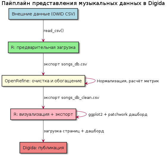
Описание исследования
Исследование посвящено анализу структурированных музыкальных метаданных на примере датасета песен из индийских фильмов.
Цель
Выявить статистически значимые связи между метаданными песен (язык, исполнитель, фильм) и их эмоциональной категорией, а также построить и валидировать модель машинного обучения для прогнозирования эмоции песни на основе доступных признаков с точностью не ниже 75% (F1-macro).
Задачи
- Выполнить предобработку: кодирование категориальных признаков (Artist, Movie, Language), балансировку данных (при необходимости), разделение на обучающую/тестовую выборки.
- Выполнить предобработку: кодирование категориальных признаков (Artist, Movie, Language), балансировку данных (при необходимости), разделение на обучающую/тестовую выборки.
- Построить и сравнить несколько моделей классификации (логистическая регрессия, Random Forest, XGBoost) с кросс-валидацией, оценить метрики качества (accuracy, precision, recall, F1-score).
- Визуализировать результаты: матрицу ошибок, важность признаков, распределение предсказаний, а также сформировать интерпретируемые выводы о доминирующих факторах, влияющих на эмоциональную окраску песни.
Гипотеза
Эмоциональная категория песни (Emotion) статистически значимо зависит от комбинации языка исполнения и исполнителя: песни на телугу в исполнении артистов «первого эшелона» (например, Sid Sriram, Armaan Malik) с большей вероятностью относятся к категориям Love или Joy, тогда как треки второстепенных исполнителей или из менее популярных фильмов чаще маркируются как Sadness или Anticipation. При этом модель, обученная на признаках Language + Artist + Movie, покажет качество прогнозирования эмоции выше базового уровня (majority class baseline) не менее чем на 20 п.п. по метрике F1-macro.
Программный код
<syntaxhighlight lang="R">
- Анализ БД
- ==========================================
- A) Imports + Global Config
- ==========================================
library(tidyverse) # dplyr, tidyr, readr, ggplot2, stringr, purrr library(lubridate) # работа с датами library(corrplot) # тепловые карты корреляций library(scales) # форматирование осей library(patchwork) # компоновка графиков
set.seed(42) options(digits = 2, width = 120)
- Глобальные настройки ggplot2
theme_set(theme_minimal(base_size = 12)) update_geom_defaults("point", list(alpha = 0.6))
- Входные параметры (аналог Python-конфига)
DATASET_NAME <- "moonknightmarvel/dataset-of-songs-with-genreartistmovielanguage" EXACT_COLUMNS <- c("title", "artist", "movie", "language", "emotion") TARGET_COL <- NULL # можно задать, например, "emotion" DATA_DIR <- "data/raw/songs_dataset.csv" # путь к файлу
- ==========================================
- B) Helper Functions (Robust & Defensive)
- ==========================================
safe_read_csv <- function(path) {
 tryCatch(
   read_csv(path, show_col_types = FALSE),
   error = function(e) {
     message(sprintf("CRITICAL ERROR: Could not read CSV at %s. Error: %s", path, e$message))
     return(tibble())
   }
 )
}
validate_columns <- function(df, expected_cols) {
 if (nrow(df) == 0 || is.null(expected_cols)) return(invisible(NULL))

 actual_cols <- names(df)
 missing <- setdiff(expected_cols, actual_cols)
 extra <- setdiff(actual_cols, expected_cols)

 cat(strrep("-", 30), "\n")
 cat(sprintf("COLUMN VALIDATION: %s\n", DATASET_NAME))

 if (length(missing) == 0 && length(extra) == 0) {
   cat("Success: All expected columns found. No extra columns.\n")
 } else {
   if (length(missing) > 0) cat(sprintf("Missing expected columns: %s\n", paste(missing, collapse = ", ")))
   if (length(extra) > 0) cat(sprintf("Extra columns found: %s\n", paste(extra, collapse = ", ")))
 }
 cat(strrep("-", 30), "\n")
 invisible(NULL)
}
audit_missingness <- function(df) {
 null_counts <- colSums(is.na(df))
 null_pct <- (null_counts / nrow(df)) * 100
 non_null <- nrow(df) - null_counts

 tibble(
   Column = names(df),
   `Null Count` = null_counts,
   `Null %` = round(null_pct, 2),
   `Non-Null Count` = non_null
 ) %>% arrange(desc(`Null %`))
}
detect_column_types <- function(df) {
 num_cols <- names(df)[sapply(df, is.numeric)]
 char_cols <- names(df)[sapply(df, is.character)]

 # Эвристика для дат: ищем паттерны вроде "2024-01-15" или "15/01/2024"
 date_pattern <- "\\d{4}-\\d{2}-\\d{2}|\\d{2}/\\d{2}/\\d{4}"
 date_cols <- char_cols[sapply(df[char_cols], function(col) {
   any(str_detect(na.omit(as.character(col[1:min(5, length(col))])), date_pattern), na.rm = TRUE)
 })]

 cat_cols <- setdiff(char_cols, date_cols)
 list(num = num_cols, cat = cat_cols, date = date_cols)
}
safe_to_numeric <- function(series) {
suppressWarnings(as.numeric(series))
}
safe_to_datetime <- function(series) {
 parsed <- parse_date_time(series, orders = c("Ymd", "dmy", "mdY"), quiet = TRUE)
 ifelse(is.na(parsed), NA, parsed)
}
plot_missingness <- function(df) {
 null_pct <- colSums(is.na(df)) / nrow(df) * 100
 null_pct <- null_pct[null_pct > 0] %>% sort(decreasing = TRUE) %>% head(30)

 if (length(null_pct) == 0) return(NULL)

 tibble(Column = names(null_pct), `Missing %` = null_pct) %>%
   mutate(Column = fct_reorder(Column, `Missing %`)) %>%
   ggplot(aes(x = `Missing %`, y = Column, fill = `Missing %`)) +
   geom_col(show.legend = FALSE) +
   scale_fill_gradient(low = "#fee0d2", high = "#cb181d") +
   labs(title = "Top Columns by Missing Percentage (%)", x = "% Missing", y = NULL) +
   theme(axis.text.y = element_text(size = 9))
}
plot_univariate_num <- function(df, num_cols) {
 cols_to_plot <- head(num_cols, 12)
 if (length(cols_to_plot) == 0) return(NULL)

 plots <- lapply(cols_to_plot, function(col) {
   df %>%
     drop_na(!!sym(col)) %>%
     ggplot(aes(x = .datacol)) +
     geom_histogram(aes(y = after_stat(density)), bins = 30, fill = "teal", color = "white", alpha = 0.8) +
     geom_density(color = "darkred", linewidth = 0.8) +
     labs(title = sprintf("Distribution of %s", col), x = NULL, y = "Density") +
     theme(axis.text.x = element_text(angle = 45, hjust = 1))
 })

 wrap_plots(plots, ncol = 3)
}
plot_univariate_cat <- function(df, cat_cols) {
 cols_to_plot <- head(cat_cols, 6)
 if (length(cols_to_plot) == 0) return(NULL)

 lapply(cols_to_plot, function(col) {
   top_vals <- df %>%
     count(.datacol, sort = TRUE) %>%
     slice_head(n = 15)

   top_vals %>%
     mutate(!!col := fct_reorder(.datacol, n)) %>%
     ggplot(aes(x = n, y = .datacol, fill = n)) +
     geom_col(show.legend = FALSE) +
     scale_fill_viridis_d(option = "viridis") +
     labs(title = sprintf("Top 15 Categories: %s", col), x = "Count", y = NULL) +
     theme(axis.text.y = element_text(size = 9))
 })
}
plot_correlation <- function(df, num_cols) {
 if (length(num_cols) < 2) return(NULL)

 corr_mat <- df %>% select(all_of(num_cols)) %>% cor(use = "complete.obs")
 corrplot(corr_mat,
          method = "color",
          type = "upper",
          tl.cex = 0.8,
          tl.srt = 45,
          addCoef.col = "black",
          number.cex = 0.6,
          col = colorRampPalette(c("#6D9EC1", "white", "#E46726"))(200),
          title = "Pearson Correlation Matrix",
          mar = c(0,0,1,0))
}
- ==========================================
- C) Load + Validate
- ==========================================
df <- safe_read_csv(DATA_DIR) validate_columns(df, EXACT_COLUMNS)
if (nrow(df) > 0) {
 # ==========================================
 # D) Data Audit
 # ==========================================
 cat(sprintf("\n--- DATA AUDIT: %s ---\n", DATASET_NAME))
 cat(sprintf("Shape: %d rows × %d columns\n", nrow(df), ncol(df)))
 cat(sprintf("Memory Usage: %.2f MB\n", object.size(df) / 1024^2))
 cat(sprintf("Duplicates: %d\n", sum(duplicated(df))))

 null_audit <- audit_missingness(df)
 cat("\nNull Audit Summary (Top 5 Missing):\n")
 print(null_audit %>% slice_head(n = 5))

 col_types <- detect_column_types(df)
 num_cols <- col_types$num
 cat_cols <- col_types$cat
 date_cols <- col_types$date

 cat(sprintf("\nDetected Numeric Columns: %s\n", paste(num_cols, collapse = ", ")))
 cat(sprintf("Detected Categorical Columns: %s\n", paste(cat_cols, collapse = ", ")))
 cat(sprintf("Detected Date Columns: %s\n", paste(date_cols, collapse = ", ")))

 # Проверка на бесконечные значения и низкую дисперсию
 if (length(num_cols) > 0) {
   inf_counts <- sum(sapply(df[num_cols], function(x) sum(is.infinite(x))), na.rm = TRUE)
   cat(sprintf("Total Inf/-Inf values: %d\n", inf_counts))

   low_var <- num_cols[sapply(df[num_cols], function(x) sd(x, na.rm = TRUE) < 0.01)]
   if (length(low_var) > 0) cat(sprintf("Low variance columns: %s\n", paste(low_var, collapse = ", ")))
 }

 # ==========================================
 # E) ETL (Safe + Reversible)
 # ==========================================
 df_clean <- df %>% mutate(across(everything(), ~.x))  # явное копирование

 # Очистка строк: пробелы + унификация пропусков
 missing_tokens <- c("", "NA", "N/A", "null", "None", "nan")
 df_clean <- df_clean %>%
   mutate(across(where(is.character), ~{
     .x %>%
       str_trim() %>%
       na_if("") %>%
       { ifelse(. %in% missing_tokens, NA, .) }
   }))

 # Попытка конвертировать "числовые" строки в numeric
 for (col in cat_cols) {
   if (col %in% names(df_clean)) {
     sample_vals <- df_cleancol %>% drop_na() %>% head(10) %>% as.character()
     if (all(str_detect(sample_vals, "^-?\\d+(\\.\\d+)?$"), na.rm = TRUE) && length(sample_vals) > 0) {
       df_cleancol <- safe_to_numeric(df_cleancol)
     }
   }
 }

 # Удаление дубликатов
 df_clean <- df_clean %>% distinct()

 # Пересчёт типов после очистки
 col_types <- detect_column_types(df_clean)
 num_cols <- col_types$num
 cat_cols <- col_types$cat

 # Обработка пропусков: импутация + индикаторы
 for (col in num_cols) {
   if (any(is.na(df_cleancol))) {
     df_cleanpaste0(col, "__was_missing") <- as.integer(is.na(df_cleancol))
     df_cleancol <- ifelse(is.na(df_cleancol),
                               median(df_cleancol, na.rm = TRUE),
                               df_cleancol)
   }
 }

 for (col in cat_cols) {
   if (any(is.na(df_cleancol))) {
     df_cleanpaste0(col, "__was_missing") <- as.integer(is.na(df_cleancol))
     df_cleancol <- replace_na(df_cleancol, "Missing")
   }
 }

 # ==========================================
 # F) EDA (Univariate & Bivariate)
 # ==========================================
 if (length(num_cols) > 0) {
   cat("\nNumeric Distribution Summary:\n")
   stats <- df_clean %>%
     select(all_of(num_cols)) %>%
     summarise(across(everything(),
                      list(mean = ~mean(., na.rm = TRUE),
                           std = ~sd(., na.rm = TRUE),
                           min = ~min(., na.rm = TRUE),
                           median = ~median(., na.rm = TRUE),
                           max = ~max(., na.rm = TRUE),
                           skew = ~mean((. - mean(., na.rm = TRUE))^3, na.rm = TRUE) / sd(., na.rm = TRUE)^3),
                      .names = "{.col}_{.fn}"))
   print(stats)

   # Поиск высококоррелирующих пар
   if (length(num_cols) >= 2) {
     corr_mat <- df_clean %>% select(all_of(num_cols)) %>% cor(use = "complete.obs") %>% abs()
     upper <- corr_mat[upper.tri(corr_mat)]
     high_corr <- which(upper >= 0.85, arr.ind = TRUE)

     if (nrow(high_corr) > 0) {
       cat("\nHighly Correlated Pairs (|r| >= 0.85):\n")
       for (i in seq_len(nrow(high_corr))) {
         row_name <- rownames(corr_mat)[high_corr[i, 1]]
         col_name <- colnames(corr_mat)[high_corr[i, 2]]
         cat(sprintf(" - %s & %s: %.3f\n", row_name, col_name, upper[high_corr[i, 1], high_corr[i, 2]]))
       }
     }
   }
 }

 # ==========================================
 # G) Feature Engineering (Lightweight)
 # ==========================================
 text_candidates <- intersect(c("title", "artist", "movie", "language"), cat_cols)

 for (col in text_candidates) {
   if (col %in% names(df_clean)) {
     df_cleanpaste0(col, "__len") <- str_length(as.character(df_cleancol))
     df_cleanpaste0(col, "__words") <-
       str_count(as.character(df_cleancol), "\\S+")  # количество слов
   }
 }

 # Раскрытие дат
 for (col in date_cols) {
   if (col %in% names(df_clean)) {
     df_cleancol <- safe_to_datetime(df_cleancol)
     if (!all(is.na(df_cleancol))) {
       df_cleanpaste0(col, "__year") <- year(df_cleancol)
       df_cleanpaste0(col, "__month") <- month(df_cleancol)
       df_cleanpaste0(col, "__dayofweek") <- wday(df_cleancol, week_start = 1)
     }
   }
 }

 # ==========================================
 # H) Visualization
 # ==========================================
 # Missingness plot
 p_missing <- plot_missingness(df)
 if (!is.null(p_missing)) print(p_missing)

 # Обновляем типы после Feature Engineering
 col_types_upd <- detect_column_types(df_clean)
 num_cols_upd <- col_types_upd$num

 # Univariate numerical
 p_num <- plot_univariate_num(df_clean, num_cols_upd)
 if (!is.null(p_num)) print(p_num)

 # Univariate categorical
 p_cat_plots <- plot_univariate_cat(df_clean, cat_cols)
 if (!is.null(p_cat_plots)) lapply(p_cat_plots, print)

 # Correlation heatmap
 plot_correlation(df_clean, num_cols_upd)

 # Target-aware analysis
 if (!is.null(TARGET_COL) && TARGET_COL %in% names(df_clean)) {
   cat(sprintf("\nTarget Analysis: %s\n", TARGET_COL))

   if (TARGET_COL %in% num_cols_upd) {
     # Числовая целевая: корреляции
     target_corr <- df_clean %>%
       select(all_of(num_cols_upd)) %>%
       cor(use = "complete.obs")[, TARGET_COL] %>%
       sort(decreasing = TRUE)
     cat("Correlations with Target:\n")
     print(target_corr)
   } else {
     # Категориальная целевая: распределение
     df_clean %>%
       count(.dataTARGET_COL, sort = TRUE) %>%
       mutate(!!TARGET_COL := fct_reorder(.dataTARGET_COL, n)) %>%
       ggplot(aes(x = n, y = .dataTARGET_COL, fill = n)) +
       geom_col(show.legend = FALSE) +
       scale_fill_viridis_d(option = "magma") +
       labs(title = sprintf("Target Distribution: %s", TARGET_COL),
            x = "Count", y = NULL) +
       theme(axis.text.y = element_text(size = 10)) %>%
       print()
   }
 }

 # ==========================================
 # I) Final Artifact Output
 # ==========================================
 cat("\n--- FINAL SUMMARY ---\n")
 cat(sprintf("Original Shape: %d × %d\n", nrow(df), ncol(df)))
 cat(sprintf("Cleaned Shape:  %d × %d\n", nrow(df_clean), ncol(df_clean)))
 cat(sprintf("Duplicates removed: %d\n", sum(duplicated(df))))
 cat(sprintf("Columns processed: %s\n", paste(names(df_clean), collapse = ", ")))
 cat("\nProcessed Data Preview (df_clean %>% head()):\n")
 print(df_clean %>% head())
} else {
message("DataFrame is empty. Pipeline terminated.")
}
- Сохранение результата (опционально)
- write_csv(df_clean, "data/processed/songs_cleaned.csv")